Johnson_DOX_24_8
Omar Johnson
2024-07-22
Last updated: 2024-07-23
Checks: 7 0
Knit directory: DOX_24_Github/
This reproducible R Markdown analysis was created with workflowr (version 1.7.1). The Checks tab describes the reproducibility checks that were applied when the results were created. The Past versions tab lists the development history.
Great! Since the R Markdown file has been committed to the Git repository, you know the exact version of the code that produced these results.
Great job! The global environment was empty. Objects defined in the global environment can affect the analysis in your R Markdown file in unknown ways. For reproduciblity it’s best to always run the code in an empty environment.
The command set.seed(20240723) was run prior to running
the code in the R Markdown file. Setting a seed ensures that any results
that rely on randomness, e.g. subsampling or permutations, are
reproducible.
Great job! Recording the operating system, R version, and package versions is critical for reproducibility.
Nice! There were no cached chunks for this analysis, so you can be confident that you successfully produced the results during this run.
Great job! Using relative paths to the files within your workflowr project makes it easier to run your code on other machines.
Great! You are using Git for version control. Tracking code development and connecting the code version to the results is critical for reproducibility.
The results in this page were generated with repository version 88c6686. See the Past versions tab to see a history of the changes made to the R Markdown and HTML files.
Note that you need to be careful to ensure that all relevant files for
the analysis have been committed to Git prior to generating the results
(you can use wflow_publish or
wflow_git_commit). workflowr only checks the R Markdown
file, but you know if there are other scripts or data files that it
depends on. Below is the status of the Git repository when the results
were generated:
Ignored files:
    Ignored:    .DS_Store
    Ignored:    analysis/Johnson_DOX_24_8.html
    Ignored:    analysis/Johnson_DOX_24_RUV_Limma.html

Untracked files:
    Untracked:  Fig_2.Rmd
    Untracked:  Fig_2.html
    Untracked:  analysis/Johnson_DOX_24_RUV_Limma.Rmd
Note that any generated files, e.g. HTML, png, CSS, etc., are not included in this status report because it is ok for generated content to have uncommitted changes.
These are the previous versions of the repository in which changes were
made to the R Markdown (analysis/Johnson_DOX_24_8.Rmd) and
HTML (docs/Johnson_DOX_24_8.html) files. If you’ve
configured a remote Git repository (see ?wflow_git_remote),
click on the hyperlinks in the table below to view the files as they
were in that past version.
| File | Version | Author | Date | Message |
|---|---|---|---|---|
| Rmd | 88c6686 | Omar-Johnson | 2024-07-23 | Publish the initial files for myproject |
Load Libraries
Read in Data
Functions
perform_module_comparisons_mutexc_2 <- function(df, module_col, value_col) {
  # Ensure the necessary columns exist
  if (!(module_col %in% names(df) && value_col %in% names(df))) {
    stop("Specified columns do not exist in the dataframe.")
  }

  # Get a list of all unique modules
  modules <- unique(df[[module_col]])

  # Initialize an empty list to store combined data frames
  combined_df_list <- list()

  # Initialize an empty dataframe to store results
  results <- data.frame(Module1 = character(),
                        Module2 = character(),
                        WilcoxPValue = numeric(),
                        stringsAsFactors = FALSE)

  # Loop through each module
  for (module in modules) {
    # Data for the current module
    current_data <- df %>% filter(!!sym(module_col) == module) %>%
                    mutate(Group = as.character(module))

    # Data for all other modules
    other_data <- df %>% filter(!!sym(module_col) != module) %>%
                    mutate(Group = paste("Not", module, sep=""))

    # Combine current module data with other module data
    combined_data <- rbind(current_data, other_data)

    # Add the combined data to the list
    combined_df_list[[module]] <- combined_data

    # Perform the Wilcoxon test
    test_result <- wilcox.test(current_data[[value_col]], other_data[[value_col]])

    # Add the results to the dataframe
    results <- rbind(results, data.frame(Module1 = module,
                                         Module2 = "Others",
                                         WilcoxPValue = test_result$p.value))
  }

  return(list("results" = results, "combined_data" = combined_df_list))
}


perform_module_disease_analysis_genes_3 <- function(toptable, diseaseGenes) {
  # Prepare an empty list to collect results
  results <- list()

  # Ensure 'Modules' and 'hgnc_symbol' columns exist in 'toptable'
  if(!"Modules" %in% names(toptable)) {
    stop("Column 'Modules' not found in the 'toptable'.")
  }
  if(!"hgnc_symbol" %in% names(toptable)) {
    stop("Column 'hgnc_symbol' not found in the 'toptable'.")
  }

  # Filter disease genes to include only those that are expressed in toptable
  expressedDiseaseGenes <- lapply(diseaseGenes, function(genes) {
    intersect(genes, toptable$hgnc_symbol)
  })

  # Loop through each module
  modules <- unique(toptable$Modules)
  for (module in modules) {
    # Get the genes in the module
    moduleGenes <- toptable$hgnc_symbol[toptable$Modules == module]

    # Loop through each disease gene set
    for (diseaseName in names(expressedDiseaseGenes)) {
      # Find the intersecting genes between the module and the expressed disease genes
      diseaseModuleIntersect <- intersect(moduleGenes, expressedDiseaseGenes[[diseaseName]])

      # Calculate elements for the contingency table
      numIntersect = length(diseaseModuleIntersect)
      numInModuleNotDisease = length(moduleGenes) - numIntersect
      numInDiseaseNotModule = length(expressedDiseaseGenes[[diseaseName]]) - numIntersect
      numInNeither = nrow(toptable) - (numIntersect + numInModuleNotDisease + numInDiseaseNotModule)

      # Build the contingency table
      table <- matrix(c(
        numIntersect, # Both in disease list and module
        numInModuleNotDisease, # In module but not disease list
        numInDiseaseNotModule, # In disease list but not module
        numInNeither # In neither list
      ), nrow = 2, byrow = TRUE)

      # Perform chi-squared test and Fisher's exact test with error handling
      chiSqTestResult <- tryCatch({
        chisq.test(table, correct = TRUE)
      }, error = function(e) {
        list(p.value = NA)
      }, warning = function(w) {
        list(p.value = NA)
      })

      fisherTestResult <- tryCatch({
        fisher.test(table)
      }, error = function(e) {
        list(p.value = NA)
      }, warning = function(w) {
        list(p.value = NA)
      })

      # Calculate percent overlap, handle division by zero
      percentOverlap <- if (length(moduleGenes) > 0) {
        (numIntersect / length(expressedDiseaseGenes[[diseaseName]])) * 100
      } else {
        0
      }

      # Convert intersecting genes to a single character string
      intersectingGenesStr <- if (numIntersect > 0) {
        paste(diseaseModuleIntersect, collapse = ";")
      } else {
        ""  # Use an empty string to indicate no intersection
      }

      # Append to results list
      results[[paste(module, diseaseName, sep = "_")]] <- data.frame(
        Modules = module,
        Disease = diseaseName,
        ChiSqPValue = chiSqTestResult$p.value,
        FisherPValue = fisherTestResult$p.value,
        PercentOverlap = percentOverlap,
        OddsRatio = fisherTestResult$estimate,
        IntersectingGenes = intersectingGenesStr
      )
    }
  }

  # Combine results into a single data frame
  results_df <- do.call(rbind, results)
  return(results_df)
}


# Function assignment
perform_fisher_test_FP <- function(vec1, vec2, vec1_name, vec2_name, plot = FALSE) {
  # Create labeled factors for vec1 and vec2
  vec1_label <- factor(vec1, labels = c(paste0("Not", vec1_name), paste0("Is", vec1_name)))
  vec2_label <- factor(vec2, labels = c(paste0("Not", vec2_name), paste0("Is", vec2_name)))

  # Create contingency table with labeled factors
  table <- table(vec1_label, vec2_label)

  # Perform Fisher's exact test
  test_result <- fisher.test(table)
  p_value <- test_result$p.value
OR <- test_result$estimate
CI <- test_result$conf.int

  # Prepare result
  result <- list(
    ContingencyTable = table,
    PValue = p_value,
    Odds_ratio = test_result$estimate,
    Confidence_Interval = test_result$conf.int
  )

  # Generate plot if required
  if (plot) {
    # Convert table to data frame for ggplot
    table_df <- as.data.frame(as.table(table))
    colnames(table_df) <- c("vec1_label", "vec2_label", "Freq")

    # Calculate totals for each vec1_label
    totals <- aggregate(Freq ~ vec1_label, data = table_df, sum)

    # Merge totals with table_df and calculate percentages
    table_df <- merge(table_df, totals, by = "vec1_label", all.x = TRUE)
    table_df$Percentage <- with(table_df, Freq.x / Freq.y * 100)
    table_df$Group <- table_df$vec2_label

    # Stacked bar chart
    p <- ggplot(table_df, aes(x = vec1_label, y = Percentage, fill = Group)) +
      geom_bar(stat = "identity", position = "stack") +  # Adjust position to "stack"
      facet_wrap(~ vec1_label) +
      theme_minimal() +
      labs(x = vec1_name, y = "Percentage", fill = vec2_name, title = paste("")) +
      theme(axis.text.x = element_text(angle = 45, hjust = 1))

    result$Plot <- p
  }

  return(result)
}


group_by_deciles <- function(x) {
  deciles <- cut(x,
                 breaks = quantile(x, probs = seq(0, 1, by = 0.1), na.rm = TRUE),
                 include.lowest = TRUE,
                 labels = paste0("D", 1:10))
  return(deciles)
}
8B-Odds of being CVD pro
BigGWASsumstat <- read_tsv(file = File_path_1)Rows: 5709 Columns: 15
── Column specification ────────────────────────────────────────────────────────
Delimiter: "\t"
chr (13): riskAllele, pValueAnnotation, riskFrequency, orValue, beta, ci, ma...
dbl (2): pValue, pubmedId
ℹ Use `spec()` to retrieve the full column specification for this data.
ℹ Specify the column types or set `show_col_types = FALSE` to quiet this message.BigGWASsumstat_sep <- separate_rows(BigGWASsumstat, mappedGenes, sep = ",")
BigGWASsumstat_sep %>% nrow()[1] 7843GWAS_Traits_to_remove <- BigGWASsumstat_sep[BigGWASsumstat_sep$mappedGenes == "-", ]$traitName %>% unique()
BigGWASsumstat_sep_filt <- BigGWASsumstat_sep[!BigGWASsumstat_sep$traitName %in% GWAS_Traits_to_remove, ]
CVD_GWAS_genes <- BigGWASsumstat_sep_filt$mappedGenes %>% unique()
GWAS_pros <- PPI_Name_Key[PPI_Name_Key$hgnc_symbol %in% CVD_GWAS_genes, ]$uniprotswissprot
pQTL_data_summary_merged <- Toptable_Modules
pQTL_data_summary_merged <- pQTL_data_summary_merged %>%
mutate(Is_hub = if_else(Toptable_Modules$Protein %in% hubs$Gene, 1, 0))
pQTL_data_summary_merged <- pQTL_data_summary_merged %>%
mutate(Is_DA = if_else(P.Value < 0.05, 1, 0))
pQTL_data_summary_merged <- pQTL_data_summary_merged %>%
mutate(Is_GWAS = if_else(Protein %in% GWAS_pros, 1, 0))
pQTL_data_summary_merged <- pQTL_data_summary_merged %>%
mutate(Is_DOXcorr = if_else((Modules %in% c("green","darkgreen","midnightblue","salmon","lightyellow")), 1, 0))
result_pLI_DOXcorr <- perform_fisher_test_FP(vec1 = pQTL_data_summary_merged$Is_DOXcorr, vec2 = pQTL_data_summary_merged$Is_GWAS, vec1_name = "DAP", vec2_name = "GWAS_Pro", plot = FALSE)
result_pLI_HUB <- perform_fisher_test_FP(vec1 = pQTL_data_summary_merged$Is_hub, vec2 = pQTL_data_summary_merged$Is_GWAS, vec1_name = "Hub", vec2_name = "GWAS_Pro", plot = FALSE)
pQTL_data_summary_merged_hubs <- pQTL_data_summary_merged[pQTL_data_summary_merged$Is_hub == TRUE, ]
result_pLI_DOX_corr_hub <- perform_fisher_test_FP(vec1 = pQTL_data_summary_merged_hubs$Is_DOXcorr, vec2 = pQTL_data_summary_merged_hubs$Is_GWAS, vec1_name = "DOXcorr hub", vec2_name = "GWAS_Pro", plot = TRUE)
FP_List <- list(result_pLI_DOX_corr_hub, result_pLI_HUB, result_pLI_DOXcorr)
FP_DF <- data.frame(
Odds_ratio = numeric(length(FP_List)),
Lower_CI = numeric(length(FP_List)),
Upper_CI = numeric(length(FP_List)),
Pval = numeric(length(FP_List))
)
for (i in 1:length(FP_List)) {
FP_DF$Odds_ratio[i] <- FP_List[[i]]$Odds_ratio
FP_DF$Lower_CI[i] <- FP_List[[i]]$Confidence_Interval[1]
FP_DF$Upper_CI[i] <- FP_List[[i]]$Confidence_Interval[2]
FP_DF$Pval[i] <- FP_List[[i]]$PValue
}
# Add row names for the labels in the forest plot
FP_DF$Label <- c("DOXcorrhub", "hub", "DOXcorr")
FP_DF$Label <- factor(FP_DF$Label, levels = rev(c( "hub", "DOXcorr", "DOXcorrhub")))
ggplot(FP_DF, aes(x = Label, y = Odds_ratio, ymin = Lower_CI, ymax = Upper_CI)) +
geom_pointrange() +
geom_hline(yintercept = 1, linetype = "dashed", color = "red") +
coord_flip() +
labs(
title = "CVD risk protein enrichment across network proteins",
x = "",
y = "Odds of being CVD protein (95% CI)"
) +
theme_classic()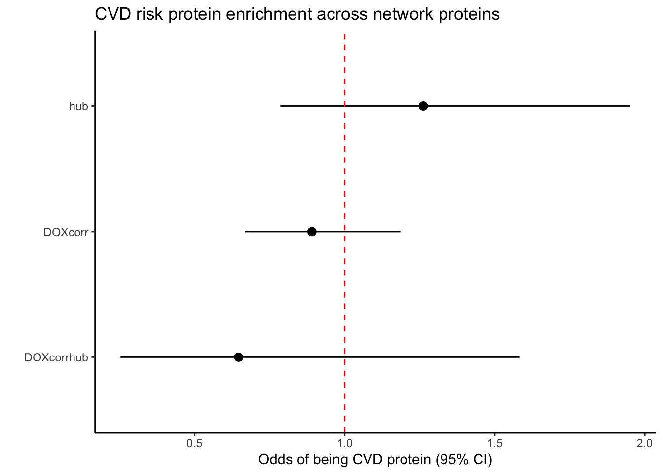
8D-Odds of being CVD-PPI
Enrichment_DF_ALL_GWASuni <- Enrichment_DF_ALL_GWASuni %>%
  mutate(Is_DOXcorr = if_else(Enrichment_DF_ALL_GWASuni$Modules %in% c("green","darkgreen","midnightblue","salmon","lightyellow"), 1, 0))

FP_DOXcorr_PPI <- perform_fisher_test_FP(vec1 = Enrichment_DF_ALL_GWASuni$Is_GWAS_PPI, vec2 = Enrichment_DF_ALL_GWASuni$Is_DOXcorr, vec1_name = "PPI with GWAS protein", vec2_name = "DOXcorr.Hub",  plot = TRUE)


FP_Hub_PPI <- perform_fisher_test_FP(vec1 = Enrichment_DF_ALL_GWASuni$Is_GWAS_PPI, vec2 = Enrichment_DF_ALL_GWASuni$Is_Hub, vec1_name = "PPI with GWAS protein", vec2_name = "DAPs",  plot = TRUE)


Enrichment_DF_ALL_GWASuni_hub <- Enrichment_DF_ALL_GWASuni[Enrichment_DF_ALL_GWASuni$Is_Hub == 1, ]

FP_DOXcorr_Hub_PPI <- perform_fisher_test_FP(vec1 = Enrichment_DF_ALL_GWASuni_hub$Is_GWAS_PPI, vec2 = Enrichment_DF_ALL_GWASuni_hub$Is_DOXcorr.Hub, vec1_name = "PPI with GWAS protein", vec2_name = "DOX Corr. hub",  plot = TRUE)


FP_List <- list(FP_DOXcorr_Hub_PPI, FP_Hub_PPI, FP_DOXcorr_PPI)

FP_DF <- data.frame(
  Odds_ratio = numeric(length(FP_List)),
  Lower_CI = numeric(length(FP_List)),
  Upper_CI = numeric(length(FP_List)),
  Pval = numeric(length(FP_List))
)

for (i in 1:length(FP_List)) {
  FP_DF$Odds_ratio[i] <- FP_List[[i]]$Odds_ratio
  FP_DF$Lower_CI[i] <- FP_List[[i]]$Confidence_Interval[1]
  FP_DF$Upper_CI[i] <- FP_List[[i]]$Confidence_Interval[2]
  FP_DF$Pval[i] <- FP_List[[i]]$PValue
}

# Add row names for the labels in the forest plot
FP_DF$Label <- c("DOXcorrhub", "hub", "DOXcorr")


FP_DF$Label <- factor(FP_DF$Label, levels = rev(c("hub", "DOXcorr", "DOXcorrhub")))

ggplot(FP_DF, aes(x = Label, y = Odds_ratio, ymin = Lower_CI, ymax = Upper_CI)) +
  geom_pointrange() +
  geom_hline(yintercept = 1, linetype = "dashed", color = "red") +
  coord_flip() +
  labs(
    title = "CVD risk protein physical interactor enrichment",
    x = "",
    y = "Odds of being physical protein interactor with CVD proteins (95% CI)"
  ) +
  theme_minimal()+
  ylim(c(0,16))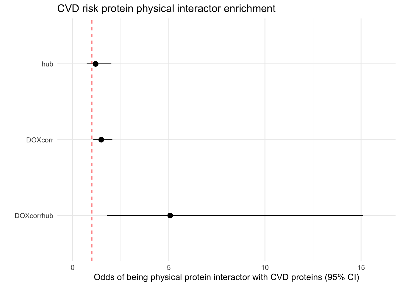
8C-CVD-pro vs CVD-PPI pLI scores
pLI_Data <- read.csv(file = File_path_2, header = TRUE)
pLI_Data_sub <- merge(pLI_Data, New_RNA_PRO_DF_3, by.x = "gene", by.y = "hgnc_symbol")
pLI_Data_sub2 <- pLI_Data_sub[,c(1,2,3)]

Toptable_Modules_pLI <- merge(Toptable_Modules, pLI_Data_sub2, by.x = "Protein" , by.y = "Protein")

# CVD protein pLI distribution
Toptable_Modules_pLI[Toptable_Modules_pLI$Is_CVD_protein == 1, ]$pLI %>% hist()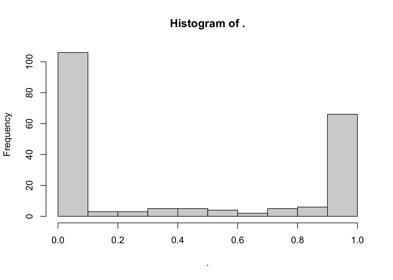
# CVD protein-PPI pLI distrbution
Toptable_Modules_pLI[Toptable_Modules_pLI$Is_CVD_PPI_protein == 1, ]$pLI %>% hist()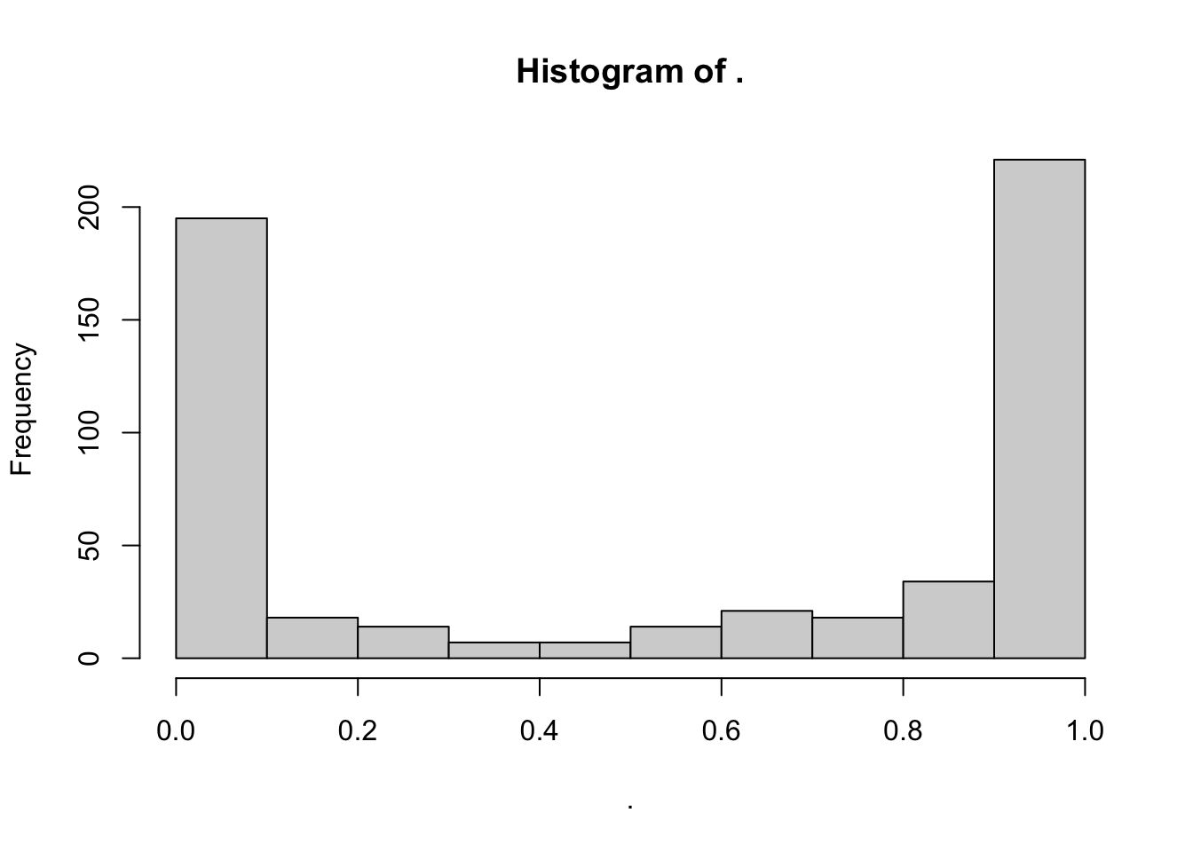
wilcox.test(Toptable_Modules_pLI[Toptable_Modules_pLI$Is_CVD_protein == 1, ]$pLI, Toptable_Modules_pLI[Toptable_Modules_pLI$Is_CVD_PPI_protein == 1, ]$pLI)
    Wilcoxon rank sum test with continuity correction

data:  Toptable_Modules_pLI[Toptable_Modules_pLI$Is_CVD_protein == 1, ]$pLI and Toptable_Modules_pLI[Toptable_Modules_pLI$Is_CVD_PPI_protein == 1, ]$pLI
W = 46186, p-value = 0.0001457
alternative hypothesis: true location shift is not equal to 0
pLI_Boxplot <- data.frame(
values = c(Toptable_Modules_pLI[Toptable_Modules_pLI$Is_CVD_protein == 1, ]$pLI,
Toptable_Modules_pLI[Toptable_Modules_pLI$Is_CVD_PPI_protein == 1, ]$pLI),
group = factor(c(rep("GWAS Pro", length(Toptable_Modules_pLI[Toptable_Modules_pLI$Is_CVD_protein == 1, ]$pLI)), rep("GWAS Pro-Interactors", length(Toptable_Modules_pLI[Toptable_Modules_pLI$Is_CVD_PPI_protein == 1, ]$pLI))))
)
# Create boxplot
ggplot(pLI_Boxplot, aes(x = group, y = values)) +
geom_boxplot() +
labs(x = "Group", y = "Mutation intolerance (pLI)") +
theme_minimal()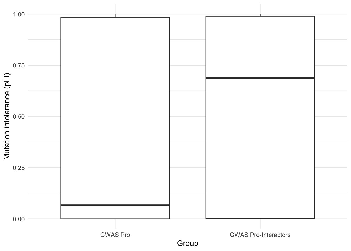
8E- CVD pro PPI network
gwas_proteins <- Toptable_Modules[Toptable_Modules$Is_CVD_protein == 1, ]$Protein

##### Net-1####
# Create the igraph object from the specific columns
g <- graph_from_data_frame(d = CVD_net[, c("query_term1", "query_term2", "Weight")], directed = FALSE)

# Annotate the graph with additional information
V(g)$is_hub <- V(g)$name %in% hubs$Gene
V(g)$is_dox_correlated <- V(g)$name %in% Toptable_Modules[Toptable_Modules$Modules %in% c("green", "darkgreen", "midnightblue", "salmon", "lightyellow"), ]$Protein
V(g)$is_cvd_pro <- V(g)$name %in% gwas_proteins

# Set vertex size based on is_hub
V(g)$size <- ifelse(V(g)$is_hub, 10, 5)  # Hubs will be larger

# Set vertex shape based on is_cvd_pro
V(g)$shape <- ifelse(V(g)$is_cvd_pro, "square", "circle")  # CVD proteins will be square

# Set vertex color based on is_dox_correlated
V(g)$color <- ifelse(V(g)$is_dox_correlated, "red", "blue")  # Dox correlated proteins will be red, others blue

# Option1
# Plot the graph
plot(g, vertex.label = NA) 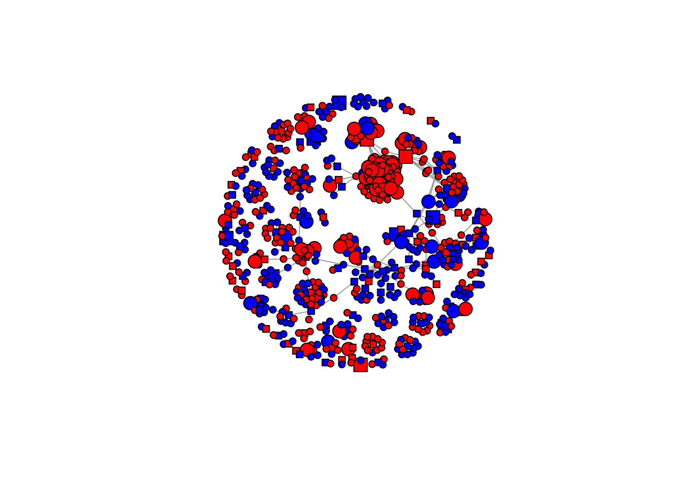
##### Net-2 #####

# Create the igraph object from the specific columns
g <- graph_from_data_frame(d = CVD_net[, c("query_term1", "query_term2", "Weight")], directed = FALSE)

# Convert igraph object to tidygraph object
tg <- as_tbl_graph(g)

# Annotate the graph with additional information
tg <- tg %>%
  mutate(is_hub = name %in% hubs$Gene,
         is_dox_correlated = name %in% Toptable_Modules[Toptable_Modules$Modules %in% c("green", "darkgreen", "midnightblue", "salmon", "lightyellow"), ]$Protein,
         is_cvd_pro = name %in% gwas_proteins,
         size = ifelse(is_hub, 10, 5),  # Hubs will be larger
         shape = ifelse(is_cvd_pro, "square", "circle"),  # CVD proteins will be square
         color = ifelse(is_dox_correlated, "red", "blue"))  # Dox correlated proteins will be red, others blue

# Plot
ggraph(tg, layout = "kk") +
  geom_edge_link0(aes(edge_color = Weight, edge_width = Weight), show.legend = TRUE) +
  geom_node_point(aes(size = size, shape = shape, color = color), show.legend = TRUE) +
  geom_node_text(aes(label = name), fontface = "bold") +
  scale_edge_color_continuous(low = "white", high = "black") +
  scale_edge_width(range = c(0.1, .2)) +
  scale_size_continuous(range = c(5, 10)) +  # Ensure the size range is the same as in the annotations
  scale_shape_manual(values = c("circle" = 16, "square" = 15)) +  # Use specific shapes
  scale_color_manual(values = c("red", "blue")) +  # Ensure the colors are used as in the annotations
  theme_graph() +
  coord_fixed()
Warning: Using the `size` aesthetic in this geom was deprecated in ggplot2 3.4.0.
ℹ Please use `linewidth` in the `default_aes` field and elsewhere instead.
This warning is displayed once every 8 hours.
Call `lifecycle::last_lifecycle_warnings()` to see where this warning was
generated.
#### Net-3 #####

# Convert igraph object to tidygraph object
tg <- as_tbl_graph(g)

# Annotate the graph with additional information
tg <- tg %>%
  mutate(is_hub = name %in% hubs$Gene,
         is_dox_correlated = name %in% Toptable_Modules[Toptable_Modules$Modules %in% c("green", "darkgreen", "midnightblue", "salmon", "lightyellow"), ]$Protein,
         is_cvd_pro = name %in% gwas_proteins,
         size = ifelse(is_hub, 10, 5),  # Hubs will be larger
         shape = ifelse(is_cvd_pro, "square", "circle"),  # CVD proteins will be square
         color = ifelse(is_dox_correlated, "red", "blue"))  # Dox correlated proteins will be red, others blue

# Define edge color based on the sign of the weight
tg <- tg %>%
  activate(edges) %>%
  mutate(edge_color = ifelse(Weight > 0, "darkgreen", "darkred"))

# Plot the graph using ggraph
ggraph(tg, layout = "kk") +
  geom_edge_link(aes(edge_color = edge_color, edge_width = abs(Weight)), show.legend = TRUE) +
  geom_node_point(aes(size = size, shape = shape, color = color), show.legend = TRUE) +
  geom_node_text(aes(label = name), fontface = "bold") +
  scale_edge_color_manual(values = c("darkgreen" = "darkgreen", "darkred" = "darkred")) +
  scale_edge_width(range = c(0.5, 2)) +  # Thicker edges
  scale_size_continuous(range = c(5, 10)) +  # Ensure the size range is the same as in the annotations
  scale_shape_manual(values = c("circle" = 16, "square" = 15)) +  # Use specific shapes
  scale_color_manual(values = c("red" = "red", "blue" = "blue")) +  # Ensure the colors are used as in the annotations
  theme_graph() +
  coord_fixed()
##### Net-4 ####
# Network with protein names

Name_Key <- read.csv(file = "/Users/omarjohnson/Downloads/idmapping_2024_07_01.csv", header = TRUE)

Toptable_Modules_key <- merge(New_RNA_PRO_DF_3,Name_Key, by.x ="Protein" , by.y = "From" )

# Create the igraph object from the specific columns
g <- graph_from_data_frame(d = CVD_net[, c("query_term1", "query_term2", "Weight")], directed = FALSE)


# Create lookup vectors for Protein to Gene name conversion
protein_to_gene <- setNames(New_RNA_PRO_DF_3$hgnc_symbol, New_RNA_PRO_DF_3$Protein)


# Replace protein names in query_term1 and query_term2 with gene names using recode
CVD_net_2 <- CVD_net %>%
  mutate(Gene1 = recode(query_term1, !!!protein_to_gene),
         Gene2 = recode(query_term2, !!!protein_to_gene))


# Select the columns with Gene names and Weight
CVD_net_3 <- CVD_net_2 %>%
  select(Gene1, Gene2, Weight)


# Create the igraph object from the specific columns
g <- graph_from_data_frame(d = CVD_net_3, directed = FALSE)

# Convert igraph object to tidygraph object
tg <- as_tbl_graph(g)


New_RNA_PRO_DF_3_hubs <- merge(New_RNA_PRO_DF_3, hubs, by.x = "Protein", by.y = "Gene")


# Annotate the graph with additional information
tg <- tg %>%
  mutate(is_hub = name %in% New_RNA_PRO_DF_3_hubs$hgnc_symbol,
         is_dox_correlated = name %in% New_RNA_PRO_DF_3[New_RNA_PRO_DF_3$Modules %in% c("green", "darkgreen", "midnightblue", "salmon", "lightyellow"), ]$hgnc_symbol,
         is_cvd_pro = name %in% CVD_GWAS_genes,
         size = ifelse(is_hub, 10, 5),  # Hubs will be larger
         shape = ifelse(is_cvd_pro, "square", "circle"),
          # CVD proteins will be square
         color = ifelse(is_dox_correlated, "red", "blue"))  # CVD proteins will be square


ggraph(tg, layout = "kk") +
  geom_edge_link0(aes(edge_color = Weight, edge_width = Weight), show.legend = TRUE) +
  geom_node_point(aes(size = size, shape = shape, color = color), show.legend = TRUE) +
  geom_node_text(aes(label = name), fontface = "bold") +
  scale_edge_color_continuous(low = "white", high = "black") +
  scale_edge_width(range = c(0.1, .2)) +
  scale_size_continuous(range = c(5, 10)) +  # Ensure the size range is the same as in the annotations
  scale_shape_manual(values = c("circle" = 16, "square" = 15)) +  # Use specific shapes
  scale_color_manual(values = c("red", "blue")) +  # Ensure the colors are used as in the annotations
  theme_graph() +
  coord_fixed()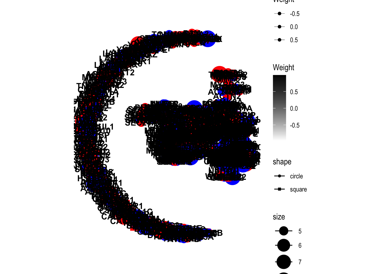
sessionInfo()R version 4.2.0 (2022-04-22)
Platform: x86_64-apple-darwin17.0 (64-bit)
Running under: macOS Big Sur/Monterey 10.16
Matrix products: default
BLAS: /Library/Frameworks/R.framework/Versions/4.2/Resources/lib/libRblas.0.dylib
LAPACK: /Library/Frameworks/R.framework/Versions/4.2/Resources/lib/libRlapack.dylib
locale:
[1] en_US.UTF-8/en_US.UTF-8/en_US.UTF-8/C/en_US.UTF-8/en_US.UTF-8
attached base packages:
[1] grid stats4 stats graphics grDevices utils datasets
[8] methods base
other attached packages:
[1] tidygraph_1.2.3
[2] igraph_1.5.1
[3] ggraph_2.1.0
[4] scales_1.2.1
[5] ReactomePA_1.40.0
[6] impute_1.70.0
[7] WGCNA_1.72-1
[8] fastcluster_1.2.3
[9] dynamicTreeCut_1.63-1
[10] BioNERO_1.4.2
[11] reshape2_1.4.4
[12] ggridges_0.5.4
[13] biomaRt_2.52.0
[14] ggvenn_0.1.10
[15] UpSetR_1.4.0
[16] DOSE_3.22.1
[17] variancePartition_1.26.0
[18] clusterProfiler_4.4.4
[19] pheatmap_1.0.12
[20] qvalue_2.28.0
[21] Homo.sapiens_1.3.1
[22] TxDb.Hsapiens.UCSC.hg19.knownGene_3.2.2
[23] org.Hs.eg.db_3.15.0
[24] GO.db_3.15.0
[25] OrganismDbi_1.38.1
[26] GenomicFeatures_1.48.4
[27] AnnotationDbi_1.58.0
[28] cluster_2.1.4
[29] ggfortify_0.4.16
[30] lubridate_1.9.2
[31] forcats_1.0.0
[32] stringr_1.5.0
[33] dplyr_1.1.2
[34] purrr_1.0.2
[35] readr_2.1.4
[36] tidyr_1.3.0
[37] tibble_3.2.1
[38] ggplot2_3.4.3
[39] tidyverse_2.0.0
[40] RColorBrewer_1.1-3
[41] RUVSeq_1.30.0
[42] edgeR_3.38.4
[43] limma_3.52.4
[44] EDASeq_2.30.0
[45] ShortRead_1.54.0
[46] GenomicAlignments_1.32.1
[47] SummarizedExperiment_1.26.1
[48] MatrixGenerics_1.8.1
[49] matrixStats_1.0.0
[50] Rsamtools_2.12.0
[51] GenomicRanges_1.48.0
[52] Biostrings_2.64.1
[53] GenomeInfoDb_1.32.4
[54] XVector_0.36.0
[55] IRanges_2.30.1
[56] S4Vectors_0.34.0
[57] BiocParallel_1.30.4
[58] Biobase_2.56.0
[59] BiocGenerics_0.42.0
[60] workflowr_1.7.1
loaded via a namespace (and not attached):
[1] rappdirs_0.3.3 rtracklayer_1.56.1 minet_3.54.0
[4] R.methodsS3_1.8.2 coda_0.19-4 bit64_4.0.5
[7] knitr_1.43 aroma.light_3.26.0 DelayedArray_0.22.0
[10] R.utils_2.12.2 rpart_4.1.19 data.table_1.14.8
[13] hwriter_1.3.2.1 KEGGREST_1.36.3 RCurl_1.98-1.12
[16] doParallel_1.0.17 generics_0.1.3 preprocessCore_1.58.0
[19] callr_3.7.3 RhpcBLASctl_0.23-42 RSQLite_2.3.1
[22] shadowtext_0.1.2 bit_4.0.5 tzdb_0.4.0
[25] enrichplot_1.16.2 xml2_1.3.5 httpuv_1.6.11
[28] viridis_0.6.4 xfun_0.40 hms_1.1.3
[31] jquerylib_0.1.4 evaluate_0.21 promises_1.2.1
[34] fansi_1.0.4 restfulr_0.0.15 progress_1.2.2
[37] caTools_1.18.2 dbplyr_2.3.3 htmlwidgets_1.6.2
[40] DBI_1.1.3 ggnewscale_0.4.9 backports_1.4.1
[43] annotate_1.74.0 aod_1.3.2 deldir_1.0-9
[46] vctrs_0.6.3 abind_1.4-5 cachem_1.0.8
[49] withr_2.5.0 ggforce_0.4.1 vroom_1.6.3
[52] checkmate_2.2.0 treeio_1.20.2 prettyunits_1.1.1
[55] ape_5.7-1 lazyeval_0.2.2 crayon_1.5.2
[58] genefilter_1.78.0 labeling_0.4.2 pkgconfig_2.0.3
[61] tweenr_2.0.2 nlme_3.1-163 nnet_7.3-19
[64] rlang_1.1.1 lifecycle_1.0.3 downloader_0.4
[67] filelock_1.0.2 BiocFileCache_2.4.0 rprojroot_2.0.3
[70] polyclip_1.10-4 graph_1.74.0 Matrix_1.5-4.1
[73] aplot_0.2.0 NetRep_1.2.7 boot_1.3-28.1
[76] base64enc_0.1-3 GlobalOptions_0.1.2 whisker_0.4.1
[79] processx_3.8.2 png_0.1-8 viridisLite_0.4.2
[82] rjson_0.2.21 bitops_1.0-7 getPass_0.2-2
[85] R.oo_1.25.0 ggnetwork_0.5.12 KernSmooth_2.23-22
[88] blob_1.2.4 shape_1.4.6 jpeg_0.1-10
[91] gridGraphics_0.5-1 reactome.db_1.81.0 graphite_1.42.0
[94] memoise_2.0.1 magrittr_2.0.3 plyr_1.8.8
[97] gplots_3.1.3 zlibbioc_1.42.0 compiler_4.2.0
[100] scatterpie_0.2.1 BiocIO_1.6.0 clue_0.3-64
[103] intergraph_2.0-3 lme4_1.1-34 cli_3.6.1
[106] patchwork_1.1.3 ps_1.7.5 htmlTable_2.4.1
[109] Formula_1.2-5 mgcv_1.9-0 MASS_7.3-60
[112] tidyselect_1.2.0 stringi_1.7.12 highr_0.10
[115] yaml_2.3.7 GOSemSim_2.22.0 locfit_1.5-9.8
[118] latticeExtra_0.6-30 ggrepel_0.9.3 sass_0.4.7
[121] fastmatch_1.1-4 tools_4.2.0 timechange_0.2.0
[124] parallel_4.2.0 circlize_0.4.15 rstudioapi_0.15.0
[127] foreign_0.8-84 foreach_1.5.2 git2r_0.32.0
[130] gridExtra_2.3 farver_2.1.1 digest_0.6.33
[133] BiocManager_1.30.22 networkD3_0.4 Rcpp_1.0.11
[136] broom_1.0.5 later_1.3.1 httr_1.4.7
[139] ComplexHeatmap_2.12.1 GENIE3_1.18.0 Rdpack_2.5
[142] colorspace_2.1-0 XML_3.99-0.14 fs_1.6.3
[145] splines_4.2.0 statmod_1.5.0 yulab.utils_0.0.8
[148] RBGL_1.72.0 tidytree_0.4.5 graphlayouts_1.0.0
[151] ggplotify_0.1.2 xtable_1.8-4 jsonlite_1.8.7
[154] nloptr_2.0.3 ggtree_3.4.4 ggfun_0.1.2
[157] R6_2.5.1 Hmisc_5.1-0 pillar_1.9.0
[160] htmltools_0.5.6 glue_1.6.2 fastmap_1.1.1
[163] minqa_1.2.5 codetools_0.2-19 fgsea_1.22.0
[166] utf8_1.2.3 sva_3.44.0 lattice_0.21-8
[169] bslib_0.5.1 network_1.18.1 pbkrtest_0.5.2
[172] curl_5.0.2 gtools_3.9.4 interp_1.1-4
[175] survival_3.5-7 statnet.common_4.9.0 rmarkdown_2.24
[178] munsell_0.5.0 GetoptLong_1.0.5 DO.db_2.9
[181] GenomeInfoDbData_1.2.8 iterators_1.0.14 gtable_0.3.4
[184] rbibutils_2.2.15